Disjoint-Sets and Agglomerative Clustering

As part of an exercise I recently to implemented agglomerative clustering for a small set of news articles. After fiddling around for a while it occurred to me that the solution would be much more elegant if cluster membership was tracked with a disjoint-set. In fact it turns out that the data structure is quite commonly used to solve this particular problem.

Agglomerative clustering is a hierarchical clustering method that starts from the ‘bottom up’. Each element initially forms its own cluster, with the nearest two clusters being progressively merged until only one remains.

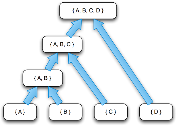example cluster One potential clustering of {A, B, C, D}, represented as a binary tree. Each level is a stage in the clustering process. Elements are missing from a level in the tree when their cluster is unchanged.

This could be more formally expressed as:

1. Let each element x in set 𝐂 be a singleton cluster
2. Until |𝐂| = 1:
	2.1 Remove two most similar clusters (x₁, x₂)
	2.2 Join to create new cluster (xₐ)
	2.3 Insert xₐ into 𝐂

Of course the main issue with this approach is efficiently finding similar clusters, which (optimistically) could take Ο(n²) time. But an important secondary issue relates to the need for a data structure to track cluster membership. A simple approach would be to use map element_id → cluster_id however this does not adequately handle the case where the two elements being merged are part of larger clusters, which would in turn also require merging.

Disjoint-sets provide a ready-made solution to this problem. The data structure maintains a collection of non-overlapping (disjoint) sets, each of which is represented by some member of that set. They can be used in a wide variety of contexts but are particularly popular with graph problems such as finding the minimum spanning tree or strongly connected components.

Three basic operations are supported by disjoint-sets:

make_set(x) creates a new set containing only x
union(x, y) combines x and y into a single set
find(x) identifies the set to which x belongs

Because of the importance of union(x, y) and find(x), disjoint-sets are sometimes referred to as union-find data structures.

Disjoint-sets, like the initial hash table approach, can be implemented as a mapping of element → subset. A particular subset is uniquely identified by the root element in the tree representing that subset. And an element is a root element if it is its own parent.

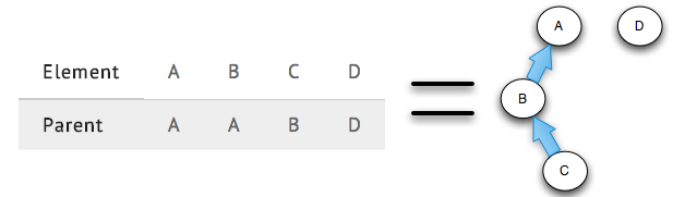disjoint set representation An example of {A, B, C, D} at after the second merge. Only {A, B, C} and {D} remain.

In a neat bit of symmetry with bottom-up clustering, disjoint-sets are initialised by calling make_set on each element.

def make_sets(x):
    return dict([(i, i) for i in x])

To find the set to which a particular element belongs, we recursively look for the parent until we find a node that is its own parent.

def find(x, parent):
    if parent[x] == x:
        return x
    else:
        return find(parent[x], parent)

To merge two existing elements, we simply find the parents of the two elements and change one to be the parent of the other.

def union(x, y, parent):
    parent[find(x, parent)] = find(y, parent)

We can even use some Python magic to find all subsets by grouping them according to their representative element.

def subsets(x):
    return itertools.groupby(x, lambda i: find(i, x))

The above Python implementation of disjoint-sets is very simple but it can nonetheless be directly applied to the agglomerative clustering problem. In which case we call make_sets(𝐂) in step 1 and union(x₁, x₂) in lieu of steps 2.2 and 2.3 of the original algorithm.

More efficient disjoint-set implementations introduce optimisations such as path compression, which speeds up the Find operation by reducing the height of the tree. This leads to an amortised complexity of Ο(log₂n). To take advantage of these performance gains, I ended up using an existing disjoint-set implementation by Ahmed El Deeb for my project.

That said, the specific paths formed by the Union function could be used to reconstruct the history of the clustering hierarchy and therefore might be worth leaving untouched. Otherwise it would be necessary to dump a copy of the subsets before each merge in order to make use of the cluster topology. Ultimately the trade off is between increased computation time (longer traversals) and memory (storing intermediate clusterings) with the former generally scarcer on modern computers.